Problem Set 9 (beta version)

$$\DeclareMathOperator*\trace{Tr} \DeclareMathOperator*\argmax{argmax} \DeclareMathOperator*\argmin{argmin} \DeclareMathOperator*\prob{\mathbb{P}}$$

This pset is ungraded. The exercises are for review purposes.

Unfolding in time

Define a recurrent net by $\begin{align} \vec{h}_{t} &= f (W \vec{h}_{t - 1} + U \vec{x}_t)\\ \vec{y}_{t} &= g (V\vec{h}_t) \end{align}$ for $t=1$ to $T$ with initial condition $\vec{h}_{0} =0$. At time $t$,

• $\vec{x}_t$ is the $d_x$-dimensional activity vector for the input neurons (input vector),
• $\vec{h}_t$ is the $d_h$-dimensional activity vector for the hidden neurons (hidden state vector),
• and $\vec{y}_t$ is the $d_y$-dimensional activity vector for the output neurons (output vector).

The network contains three connection matrices:

• The $d_h\times d_x$ matrix $U$ specifies how the hidden neurons are influenced by the input,
• the $d_h\times d_h$ “transition matrix” $W$ governs the dynamics of the hidden neurons,
• and the $d_y\times d_h$ matrix $V$ specifies how the output is “read out” from the hidden neurons.

The network can be depicted as

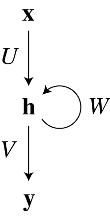
where the recurrent connectivity is represented by the loop. Note that if $W$ were zero, this would reduce to a multilayer perceptron with a single hidden layer.

If we want to run the recurrent net for a fixed number of time steps, we can unfold or unroll the loop in the above diagram to yield a feedforward net with the architecture:

$$\require{AMScd} \begin{CD} @. \vec{x}_1 @. \vec{x}_2 @. \cdots @. \vec{x}_T\\ @. @VU_1VV @VU_2VV @VVV @VU_TVV\\ \vec{h}_0 @>W_1>> \vec{h}_1 @>W_2>> \vec{h}_2 @>>> \cdots @>W_T>> \vec{h}_T\\ @. @V{V_1}VV @V{V_2}VV @VVV @V{V_T}VV\\ @. \vec{y}_1 @. \vec{y}_2 @. \cdots @. \vec{y}_T\\ \end{CD}$$

In this diagram, we temporarily imagine that the connection matrices $W_t$, $U_t$, and $V_t$ vary with time: $\begin{align} \vec{h}_{t} &= f (W_t \vec{h}_{t - 1} + U_t \vec{x}_t)\\ \vec{y}_{t} &= g (V_t\vec{h}_t) \end{align}$ This reduces to the recurrent net in the case that $W_t=W$ for all $t$ (and similarly for the other connection matrices). This is called “weight sharing through time.”

The diagram has the virtue of making explicit the pathways that produce temporal dependencies. The last output $\vec{y}_T$ depends on the last input $\vec{x}_T$ through the short pathway that goes through $\vec{h}_T$. The last output also depends on the first input $\vec{x}_1$ through the long pathway from $\vec{h}_1$ to $\vec{h}_T$.

Backpropagation through time

The backward pass can be depicted as

$$\require{AMScd} \begin{CD} @. \tilde{\vec{x}}_1 @. \tilde{\vec{x}}_2 @. \cdots @. \tilde{\vec{x}}_T\\ @. @A{U_1^\top}AA @A{U_2^\top}AA @AAA @A{U_T^\top}AA\\ \tilde{\vec{h}}_0 @<{W_1^\top}<< \tilde{\vec{h}}_1 @<{W_2^\top}<< \tilde{\vec{h}}_2 @<<< \cdots @<{W_T^\top}<< \tilde{\vec{h}}_T\\ @. @A{V_1^\top}AA @A{V_2^\top}AA @AAA @A{V_T^\top}AA\\ @. \tilde{\vec{y}}_1 @. \tilde{\vec{y}}_2 @. \cdots @. \tilde{\vec{y}}_T\\ \end{CD}$$

Here $\tilde{\vec{h}}_t$ is the backward pass variable that corresponds with the forward pass preactivity $f^{-1}(\vec{h}_t)$ (and similarly for other tilde variables).

Exercises

1. Write the equations of the backward pass corresponding to the diagram. As a concrete example, use the loss \[ E = \sum_{t=1}^T \frac{1}{2}|\vec{d}_t - \vec{y}_t|^2 \] where $\vec{d}_t$ is a vector of desired values for the output neurons at time $t$. The equations for $\tilde{\vec{x}}_t$ and $\tilde{\vec{h}}_0$ won’t be used in the gradient descent updates, but write them anyway. (They would be useful if $\vec{x}^t$ were the output of other neural net layers and we wanted to continue backpropagating through those layers too.)

2. In the gradient descent updates, $\begin{align} \Delta U_t &\propto \tilde{\vec{h}}_?\vec{x}_?^\top\\ \Delta W_t &\propto \tilde{\vec{h}}_?\vec{h}_?^\top\\ \Delta V_t &\propto \tilde{\vec{y}}_?\vec{h}_?^\top \end{align}$ supply the missing letters where there are question marks. Note how the backward pass diagram above shows the paths by which the loss at time $t$ can influence the gradient updates for previous times.

3. To obtain the backprop update for the recurrent net, we must enforce the constraint of weight sharing in time ($W_t=W$ for all $t$, etc.). Write the gradient updates for $U$, $V$, and $W$.

Backprop with multiplicative interactions

Consider the feedforward net, $\begin{align} \vec{x}^1 &= f(W^{1x}\vec{x}^0 + \vec{b}^{1x})\\ \vec{y}^1 &= f(W^{1y}\vec{y}^0 + \vec{b}^{1y})\\ \vec{z}^1 &= \vec{x}^1.*\vec{y}^1\\ \vec{z}^2 &= f(W^2\vec{z}^1 + \vec{b}^2) \end{align}$ The vectors represent the layer activities, and superscripts indicate layer indices. The elementwise multiplication of $\vec{x}^1$ and $\vec{y}^1$ makes this net different from a multilayer perceptron.

Exercises

1. Write the backward pass for the net.
2. Write the gradient updates for the weights and biases.

REINFORCE

Suppose that the probability that a random variable $X$ takes on the value $x$ is given by the parametrized function $p_\theta(x)$,

$$\prob[X = x] = p_\theta(x)$$

I am following the convention that random variables (e.g. $X$) are written in upper case, while values (e.g. $x$) are written in lower case.

Given a reward function $r(X)$, define its expected value by

$$\begin{equation}\label{eq:ExpectedReward} \langle r(X)\rangle = \sum_x p_\theta(x) r(x) \end{equation}$$

where the sum is over all possible values $x$ of the random variable $X$. The expected reward is a function of the parameters $\theta$. How can we maximize this function?

The REINFORCE algorithm consists of the following steps

• Draw a sample $x$ of the random variable $X$.
• Compute the eligibility (for reinforcement)

$$\begin{equation}\label{eq:Eligibility} e_\theta(x) = \nabla_\theta\log p_\theta(x) \end{equation}$$

• Observe the reward $r(x)$.
• Update the parameters via

$$\begin{equation}\label{eq:ThetaUpdate} \Delta\theta \propto r(x)e_\theta(x) \end{equation}$$

The basic theorem is that this algorithm is stochastic gradient ascent on the expected reward of Eq. (\ref{eq:ExpectedReward}). To apply the REINFORCE algorithm,

• It is sufficient to observe reward from random samples; no explicit knowledge of the reward function is necessary.
• One must have enough knowledge about $p_\theta(x)$ to be able to compute the eligibility.

As a special case, suppose that $X=(S,A)$ is a state-action pair taking on values $x=(s,a)$. The reward $r(S,A)$ is a function of both state and action, and the probability distribution of state-action pairs is

$$\prob[X=x] = \prob[S=s, A=a] = \prob[S=s]\prob[A=a|S=s]$$

We interpret the probability \(\prob[S=s]\) as describing the states of the world. The conditional probability \(\log\prob[A=a|S=s]\) describes a stochastic machine that takes the state \(S\) of the world as input and produces action \(A\) as output. So the eligibility is

$$\nabla_\theta\log\prob[X=x] = \nabla_\theta\log\prob[S=s] + \nabla_\theta\log\prob[A=a|S=s]$$

The first term in the sum vanishes because the parameter $\theta$ does not affect the world. Therefore we can be ignorant of $\prob[S=s]$, which is fortunate given that the world is complex. Only the second term in the sum matters, because $\theta$ only affects the stochastic machine. So the eligibility reduces to

$$\nabla_\theta\log\prob[X=x] = \nabla_\theta\log\prob[A=a|S=s]$$

We’ve only considered the case in which successive states of the world are drawn independently at random. It turns out that REINFORCE easily generalizes to control of a Markov decision process, in which states of the world have temporal dependences. It also generalizes to partially observable Markov decision processes, in which the stochastic machine has incomplete information about the state of the world.

REINFORCE-backprop

Suppose that the stochastic machine is a neural net with a softmax output. The parameter vector \(\theta\) then refers to the weights and biases. Note that \(\log\prob[A=a|S=s]\) is the same (up to a minus sign) as the loss function used for neural net training, assuming that the desired output is \(a\) (see softmax exercise in Problem Set 1). So \(\nabla_\theta\log\prob[A=a|S=s]\) should be the same as the backprop updates assuming that the desired output is \(a\). The minus sign doesn't matter because here we are performing stochastic gradient ascent rather than stochastic gradient descent. Therefore we can combine REINFORCE and backprop in the following algorithm

• Draw a sample $s$ of the random variable $S$ (observe the world).
• Feed $s$ as input to a neural network with a softmax output.
• Choose a random action $a$ by sampling from the softmax probability distribution.
• Pretend that the chosen action $a$ is the correct one, and compute the regular backprop updates for the weights and biases.
• Observe the reward $r$.
• Before applying the incremental updates to the weights and biases, multiply the updates by the reward $r$.

Exercises

1. Prove that Eq. (\ref{eq:ThetaUpdate}) is stochastic gradient ascent on the expected reward of Eq. (\ref{eq:ExpectedReward}). In other words, show that the expectation value of the right hand side of Eq. (\ref{eq:ThetaUpdate}) is equal to $\nabla_\theta\langle r(X)\rangle$.

2. Prove that the eligibility of Eq. (\ref{eq:Eligibility}) has zero mean. This means that the eligibility is like a “noise” that is intrinsic to the system. Note that statisticians refer to the eligibility as the score function, which is used to define Fisher information.

3. Prove that the gradient of the expected reward is the covariance of the reward and the eligibility.

4. Consider a multilayer perceptron with a single hidden layer (two layers of connections) and a final softmax output. Write out the REINFORCE-backprop algorithm in full.